


Momentum in the Indian Market

Buy winners and sell losers - the simplest interpretation of momentum investing. So simple, that you might doubt its effectiveness. Yet, it has stood the test of time across markets and market regimes. Momentum strategies produce significant positive alpha, especially in bull markets where it outperforms all other factors as explained by Blitz (2023).
I spent some time exploring momentum returns in the Indian market focusing on the NIFTY 50. First, I explore a strategy where we use momentum-based signals to foresee market downturns and allocate to gold. I've used NIFTYBEES and GOLDBEES ETFs to back-test this strategy.
Getting Data:
niftybees = yf.download("NIFTYBEES.BO", start="2000-01-01", end="2025-01-09", interval="1mo")
goldbees = yf.download("GOLDBEES.BO", start="2000-01-01", end="2025-01-09", interval="1mo")

niftybees = niftybees["Adj Close"]['NIFTYBEES.BO']
goldbees = goldbees["Adj Close"]['GOLDBEES.BO']['2010-03-01':]
Strategy:
The strategy is driven by 2 momentum indicators:
o Short Term Momentum momentum ratio (lagged 1 month)
o Long Term Momentum momentum ratio (lagged 1 month)
Signal:
if (short-term momentum ratio > 0 OR long-term momentum ratio > 0):
Allocate 100% to NIFTYBEES
else:
Allocate 100% to GOLDBEES
data = pd.concat([niftybees, goldbees], axis=1).dropna()

data.columns = ["NIFTYBEES", "GOLDBEES"]

# data['lagged_1_year_avg_pe'] = data['P/E'].rolling(12).mean()

# data = data['2014-11-01':'2021-03-01']

short_term_momentum_months = [1,2,3,4,5,6]
long_term_momentum_months = [6,7,8,9,10,11,12]

data["NIFTYBEES_Return"] = data["NIFTYBEES"].pct_change()
data["GOLDBEES_Return"] = data["GOLDBEES"].pct_change()

cummulative_column_names = []
return_column_names = []

for short_term_window in short_term_momentum_months:
    for long_term_window in long_term_momentum_months:
        short_term_column_name = 'lagged_' + str(short_term_window) + 'month' + '_momentum_short'
        long_term_column_name = 'lagged_' + str(long_term_window) + 'month' + '_momentum_long'

        data[short_term_column_name] = data['NIFTYBEES'].shift(1)/data['NIFTYBEES'].shift(short_term_window+1)
        data[long_term_column_name] = data['NIFTYBEES'].shift(1)/data['NIFTYBEES'].shift(long_term_window+1)

        # data = data.iloc[long_term_window+1:]
        # Generate signals
        signal_column_name = str(short_term_window) + '_' + str(long_term_window)
        data[signal_column_name] = np.where((data[short_term_column_name] > 1) | (data[long_term_column_name] > 1), "NIFTYBEES", "GOLDBEES")
Intuition:
o If short term returns are positive or long term returns are positive for NIFTY 50, allocate to NIFTY 50.
o Allocate to GOLD only when both short and long term returns are negative.
Results and Performance
We back-test the performance of different windows sizes for short-term and long-term momentum signals.
# Calculate returns
strategy_column_name = str(short_term_window) + '_' + str(long_term_window) + '_' + 'return'
        data[strategy_column_name] = np.where(
            data[signal_column_name] == "NIFTYBEES",

data["NIFTYBEES_Return"], data["GOLDBEES_Return"]
            )
        strategy_cummulative_column_name = strategy_column_name + 'cummulative'
        data[strategy_cummulative_column_name] = (1 + data[strategy_column_name]).cumprod()
        cummulative_column_names.append(strategy_cummulative_column_name)
        return_column_names.append(strategy_column_name)
Performance of 1-month short-term windows

Performance of 2-month short-term windows

Performance of 3-month short-term windows

Performance of 4-month short-term windows

Performance of 5-month short-term windows
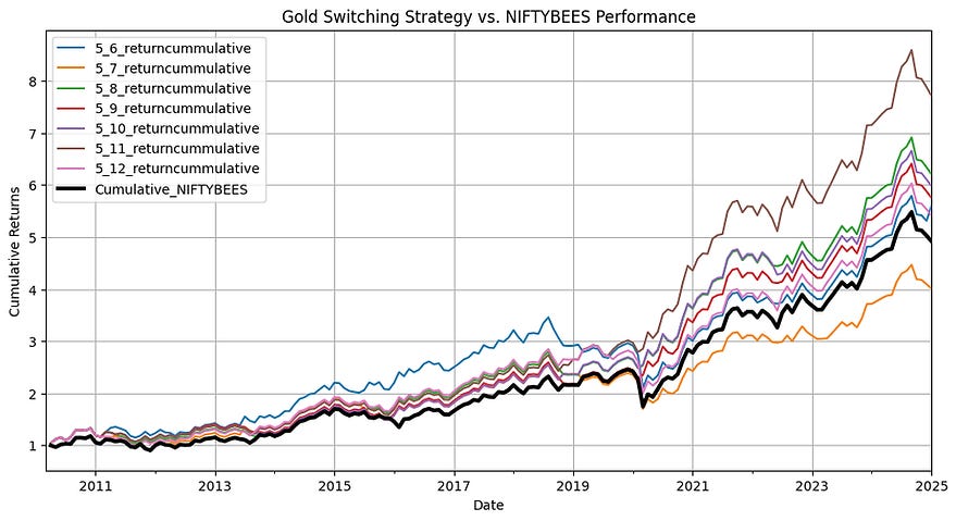
Performance of 6-month short-term windows

Getting Risk-free rate Historical Data
risk_free = pd.read_csv("risk_free_rate_india.csv")
risk_free['Date'] = pd.to_datetime(risk_free['Date'], format='%d-%m-%Y')
risk_free.set_index('Date', inplace=True)
data_metrics = pd.merge(data, risk_free, left_index=True, right_index=True , how='inner')
data_metrics = data_metrics.rename(columns={'Price': 'risk_free'})
data_metrics['risk_free'] = data_metrics['risk_free']/(100*12)
Calculating Performance Metrics for Strategies
########## Strategy Metrics

performance_df = pd.DataFrame()

for i, return_column_name in enumerate(return_column_names):
    cum_ret_column_name = cummulative_column_names[i]

    # Sharpe ratio
    sharpe_ratio = (data_metrics[return_column_name] - data_metrics['risk_free']).mean() / (data_metrics[return_column_name] - data_metrics['risk_free']).std()

    # Maximum drawdown
    rolling_max = data_metrics[cum_ret_column_name].cummax()
    drawdown = (data_metrics[cum_ret_column_name] - rolling_max) / rolling_max
    max_drawdown = drawdown.min()

    # Performance metrics
    performance = {
        "Strategy": return_column_name,
        "Sharpe Ratio": sharpe_ratio*np.sqrt(12),
        "Max Drawdown": max_drawdown,
        "Cumulative Return": data_metrics[cum_ret_column_name].iloc[-1]
    }

    print("\n")
    # Print results
    print("Performance Metrics:")
    for metric, value in performance.items():
        if isinstance(value, str):
            print(f"{metric}: {value}")
        else:
            print(f"{metric}: {value:.2f}")

    performance_df = pd.concat([performance_df, pd.DataFrame([performance])])
Using Momentum to Predict Market Drawdowns
I created a random forest model trained on momentum features created from 30+ years of monthly NIFTY 50 returns. It uses 1, 3, 6, 9, and 12 month momentum as predictors for next month market returns. It predicts whether NIFTY 50 could fall by more than 2% next month.
def get_market_data():
    DATA_FILENAME = Path(__file__).parent/'data/NIFTY 50_Historical_PR_01021990to06022025.csv'

    nifty_historical = pd.read_csv(DATA_FILENAME)
    nifty_historical['Date'] = pd.to_datetime(nifty_historical['Date'])
    nifty_historical = nifty_historical.set_index('Date').resample('ME').ffill()
    nifty_historical = nifty_historical[:'2007-10-01']
    nifty_historical  = pd.DataFrame(nifty_historical['Close'])
    nifty_historical = nifty_historical.rename(columns = {'Close': '^NSEI'})


    # Define ticker and date rangticker = "BSE-500.BO"
    start_date = "1980-01-01"
    end_date = datetime.today().strftime('%Y-%m-%d')
    ticker = '^NSEI'
    # Download data
    data = yf.download(ticker, start=start_date, end=end_date, interval="1d")
    last_date_data = data.index[-1]
    # Keep only the closing prices
    data = data[['Close']]
    yf_market_data = data['Close'].resample('ME').last()
    market_data = pd.concat([nifty_historical, yf_market_data], axis=0)

    return market_data, last_date_data

def create_momentum_features(market_data):
    windows = [1, 3, 6, 9, 12]

    market_data['momentum_1_1'] = market_data['^NSEI'] / market_data['^NSEI'].shift(1)
    market_data['momentum_3_1'] = market_data['^NSEI'] / market_data['^NSEI'].shift(3)
    market_data['momentum_6_1'] = market_data['^NSEI'] / market_data['^NSEI'].shift(6)
    market_data['momentum_9_1'] = market_data['^NSEI'] / market_data['^NSEI'].shift(9)
    market_data['momentum_12_1'] = market_data['^NSEI'] / market_data['^NSEI'].shift(12)

def train_model(market_data):
    initial_value = 100
    market_data['Return'] = market_data['^NSEI'].pct_change()
    market_data['Portfolio'] = initial_value * (1 + market_data['Return']).cumprod()
    market_data['Portfolio'].iloc[0] = initial_value
    market_data['next_month_return'] = market_data['Return'].shift(1)
    market_data.dropna(inplace=True)
    market_data['positive_returns'] = (market_data['next_month_return'] > -0.02).astype(int)

    X_final = market_data[['momentum_1_1', 'momentum_3_1', 'momentum_6_1', 'momentum_9_1', 'momentum_12_1']].iloc[:-1]
    y_final = market_data['positive_returns'].iloc[:-1]

    # Initialize the Random Forest Classifier
    clf = RandomForestClassifier(n_estimators=10, random_state=42)

    # Define k-fold cross-validation (-fold)
    kfold = StratifiedKFold(n_splits=5, shuffle=False)

    # Perform cross-validation
    cv_scores = cross_val_score(clf, X_final, y_final, cv=kfold, scoring='accuracy')

    # Train the model
    clf.fit(X_final, y_final)

    return cv_scores, clf

    # Output results
    # print(f"Cross-Validation Scores: {cv_scores}")
    # print(f"Mean Accuracy: {np.mean(cv_scores):.4f}")
    # print(f"Standard Deviation: {np.std(cv_scores):.4f}")

def make_predictions(clf, market_data):
    last_month = np.array(market_data[['momentum_1_1', 'momentum_3_1', 'momentum_6_1', 'momentum_9_1', 'momentum_12_1']].iloc[-1]).reshape(1,-1)
    final_prediction = clf.predict(last_month)

    return final_prediction
You can use my Web App to see live predictions for the next month, updated automatically with latest data.