Constructing a Quantitative Factor Portfolio for the Indian Market

The intersection of size, value, quality and momentum.

The outperformance of size, value, quality and momentum factors is well-researched and documented. A lot of research further delves into the performance of each factor in different market regimes, business cycles, and macro conditions.

I want to keep things simple. I think that with creating any strategy - it is really about where you draw the line for how much complexity you want to add and that should depend on whether the extra complexity is adding any marginal value - any improvement to risk-adjusted returns in a robust back-test?

I don’t think there is much value in trying to time factors and then trying to get it right every time. For that, you would first need models to accurately classify market regimes, business cycles, and identify relationships between macro variables and factor returns.

In my strategy - I only do two things - avoid large drawdowns during bear markets and maximize returns during bull markets. During bear markets, we sell Indian equities and allocate to a portfolio of foreign equities, gold, and government debt.

This article focuses on the construction of the factor portfolios to which we will allocate when our regime prediction model does not predict a large drawdown. We will create a portfolio of 20 stocks which will be updated every month.

We use the following factors to pick the 20 stocks:

1. Momentum

2. Quality

3. Value

Also, we do not use these factors separately to identify and rank stocks, instead we use an aggregate score based on the combination of these factors to create a single ranking system. The following section defines the step-by-step process to create the portfolio.

Step 1: Defining the universe of stocks to pick from

We use the following rules on Trendlyne’s screener to create our universe of stocks:

Market Capitalization > 5000 AND

EV Per EBITDA Annual > 0 AND

Half Yr Change % > - 20

These filters remove bad companies that we deem too risky for our portfolio. The market cap filter removes small companies, and the half year price change removes companies that have recently seen big drops - which is a price indicator of something problematic happening with the company.

Step 2: Defining data points to create factor signals

We need the following data points to create factor signals and remove some companies based on accounting red flags:

Step 3: Defining factor signals

First, we scale all factor outputs using standard normal scaling, x' = (x - μ) / σ.

Momentum Signal: Average of scaled 6-month and 12-month price returns

Quality Signal: Average of scaled 3-year Net Profit Growth and Last Quarter Operating Profit Margin

Value Signal: Average of scaled EBITDA / EV and scaled E/P

df['EBITDA/EV'] = 1/df['EV Per EBITDA Annual']
df['E/P'] = 1/df['PE TTM Price to Earnings']

factor_columns = ['EBITDA/EV', 'E/P', 'Half Yr Change %', '1Yr change %', 'Net Profit 3Yr Growth %', 'Operating Profit Margin Qtr %']

for factor_column in factor_columns:
    df[factor_column + '_scaled'] = (df[factor_column] - df[factor_column].mean()) / df[factor_column].std()

df['value_aggregate'] = (df['EBITDA/EV_scaled'] + df['E/P_scaled']) / 2
df['momentum_aggregate'] = (df['Half Yr Change %_scaled'] + df['1Yr change %_scaled'])/2
df['quality_aggregate'] = (df['Net Profit 3Yr Growth %_scaled'] + df['Operating Profit Margin Qtr %_scaled'])/2
df['aggregate_factor_score'] = (df['value_aggregate'] + df['momentum_aggregate'] + df['quality_aggregate'])/3

df.head()

Step 4: Removing outliers

We have already filtered for outliers based on momentum ( < -20% 6-month return). Now we use an accounting red flag to remove outliers. It is defined as follows:

STA = (net income – cash flow from operations) / Total Assets

The intuition, as borrowed from ‘The Quantitative Value Investing Philosophy’ [5], is that:

CFO (cash flow from operations), as a measure of performance, is less subject to distortion than is the net income figure. This is so because the accrual system, which produces the income number, relies on accruals, deferrals, allocations and valuations, all of which involve higher degrees of subjectivity than what enters the determination of CFO. That is why analysts prefer to relate CFO to reported net income as a check on the quality of that income. Some analysts believe that the higher the ratio of CFO to net income, the higher the quality of that income. Put another way, a company with a high level of net income and a low cash flow may be using income recognition or expense accrual criteria that are suspect.

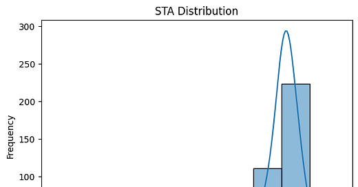
df['STA'] = (df['Net Profit Annual 1Yr Ago'] - df['Cash from Operating Activity Annual 1Yr Ago'])/df['Total Current Assets Annual 1Yr Ago']

Example distribution of STA for data from March 2025:

Finally, we remove companies that fall in the top 5 percentile of STA

# Calculate the 95th percentile threshold
percentile_95 = df['STA'].quantile(0.95)

# Filter for bottom 95% values (less than or equal to 95th percentile)
df_bottom_95 = df[df['STA'] <= percentile_95]

print("95th Percentile Threshold for STA:", percentile_95)
df_bottom_95.head()

Step 5: Factor Ranking and Portfolio

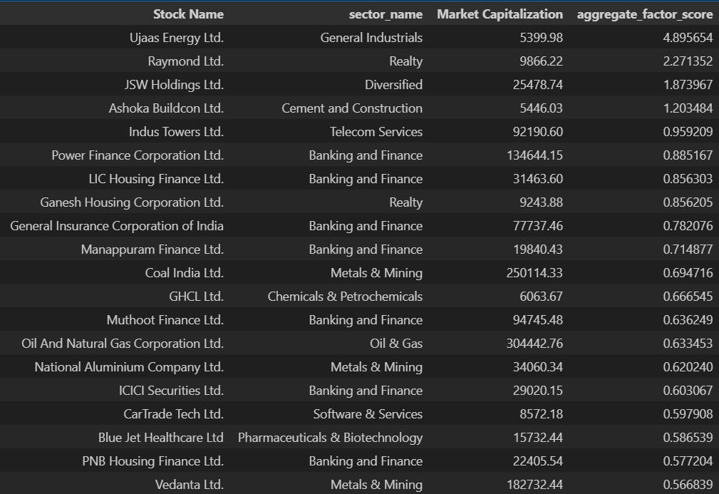
The aggregate factor score is the average of the three factor signals. Based on the aggregate factor score, we rank companies and select the top 20. Our portfolio is simple defined as an equal-weight portfolio of these 20 stocks.

df_final = df_bottom_95.sort_values('aggregate_factor_score', ascending=False)
df_final.iloc[:20][['Stock Name', 'sector_name', 'Market Capitalization', 'aggregate_factor_score']]

Example output for March 2025 data

This concludes a fairly straightforward approach that combines value, quality, and momentum to create a quantitative factor portfolio of 20 stocks.

I am yet to back-test strategy, which would require historical accounting data going back at least 10 years to evaluate the strategy over different market regimes - something which I cannot find from any free data source. This usually requires subscription to data vendors like Refinitiv (LSEG), FactSet, or Morningstar that are quite expensive for personal use.

Having said that, I plan to document the performance of this strategy going forward, which is, starting from March 2025. I also plan to further enhance this strategy by improving the outlier removal mechanism, and by defining the factors in a more sophisticated manner. So, stay tuned.

References:

1) Frazzini, Andrea and Kabiller, David and Pedersen, Lasse Heje, Buffett's Alpha (January 9, 2019). Financial Analysts Journal, 2018, 74 (4): 35-55, Available at SSRN: https://ssrn.com/abstract=3197185 or http://dx.doi.org/10.2139/ssrn.3197185

2) Asness, Cliff S. and Frazzini, Andrea and Pedersen, Lasse Heje, Quality Minus Junk (June 5, 2017). Available at SSRN: https://ssrn.com/abstract=2312432 or http://dx.doi.org/10.2139/ssrn.2312432

3) Business Cycle Sector Approach, https://www.fidelity.com/webcontent/ap101883-markets_sectors-content/18.01.0/business_cycle/Business_Cycle_Sector_Approach.pdf

4) Chen, Linda H. and Jiang, George and Zhu, Xingnong, Do Style and Sector Indexes Carry Momentum? (August 28, 2011). The Journal of Investment Strategies, vol1(3), Summer 2012, 67-89., Available at SSRN: https://ssrn.com/abstract=2139210 or http://dx.doi.org/10.2139/ssrn.2139210

5) The Quantitative Value Investing Philosophy, Wesley Gray, PhD
https://alphaarchitect.com/the-quantitative-value-investing-philosophy/

6)Blitz, David, The Cross-Section of Factor Returns (May 8, 2023). Available at SSRN: https://ssrn.com/abstract=4441376 or http://dx.doi.org/10.2139/ssrn.4441376